Appointment Timing and Daily Flow

Overview

The timing parameters check_in_time_mean and the internal appointment duration model define how early patients arrive and how long visits last.
Together, they determine the temporal flow of the simulated clinic — when patients arrive, how long they wait, and how consultations overlap throughout the day.

You will explore:

1. Typical punctuality and consultation duration patterns.

2. How late arrivals affect clinic flow and waiting times.

3. How early arrivals can improve coordination and reduce delays.

---

Example 1 – Standard punctuality and consultation time

A typical outpatient clinic where most patients arrive slightly early and sessions last around 15–20 minutes.

from medscheduler import AppointmentScheduler
from medscheduler.utils.plotting import (
    plot_arrival_time_distribution,
    plot_waiting_time_distribution,
    plot_appointment_duration_distribution
)

sched_standard = AppointmentScheduler(
    date_ranges=[("2024-01-01", "2024-03-31")],
    ref_date="2024-03-15",
    check_in_time_mean=-10,  # average 10 min early
    fill_rate=0.85
)

slots_df, appts_df, patients_df = sched_standard.generate()

# Visualizations
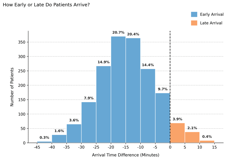
plot_arrival_time_distribution(appts_df)
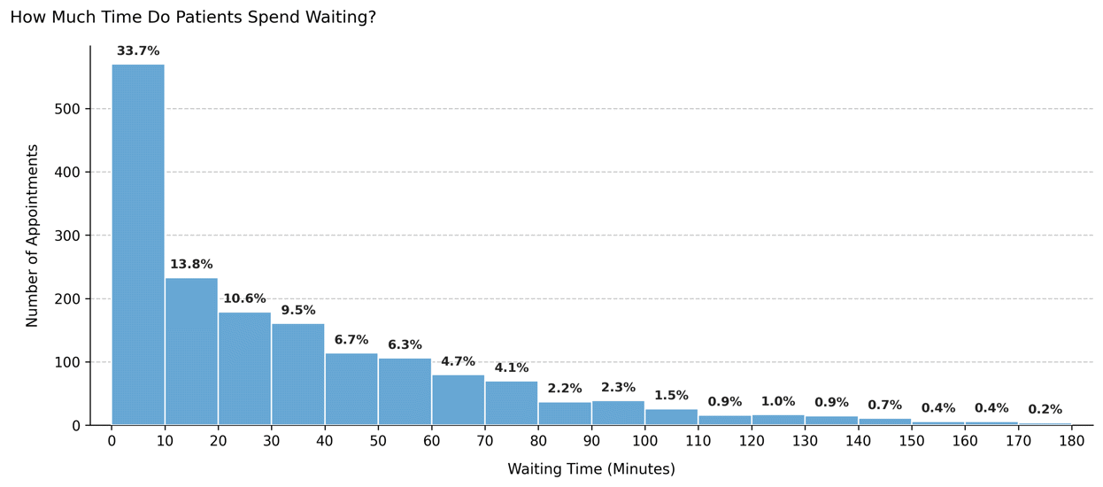
plot_waiting_time_distribution(appts_df)

Output preview:
Below are the main visualizations for this baseline scenario:

1. Arrival time distribution – Most patients check in between 5–15 minutes early.
   

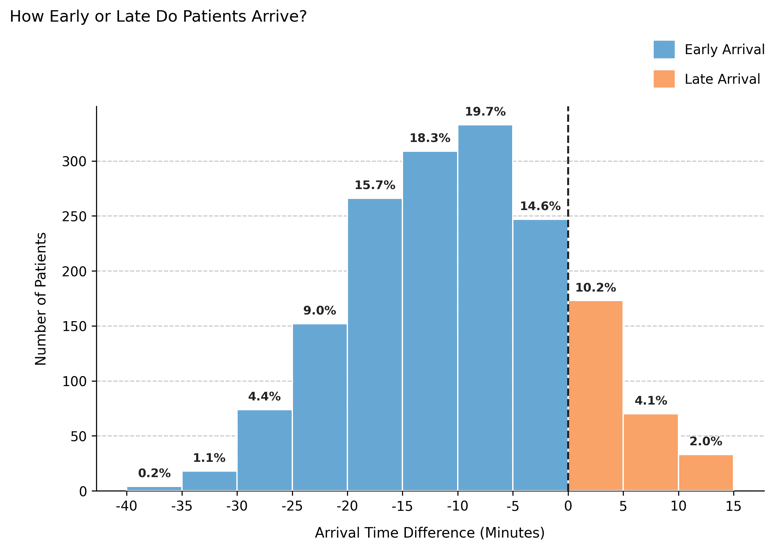
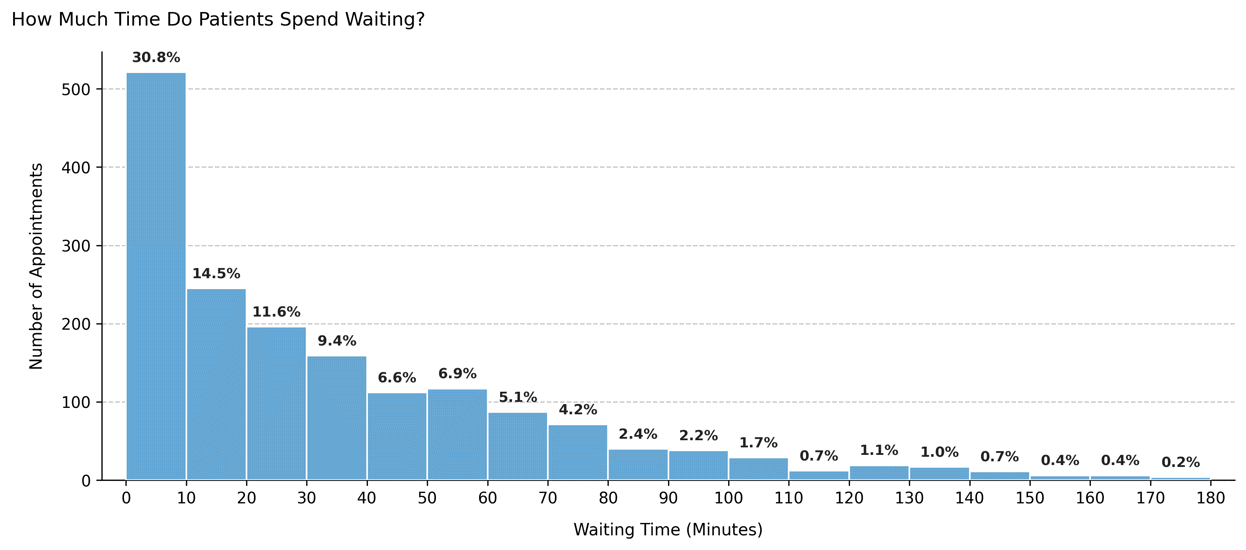
2. Waiting time distribution – Median waiting ≈ 5 minutes, showing efficient flow.

---

Appointment duration model (internal behavior)

The simulator assigns consultation durations to attended visits using a fixed stochastic model — not a user parameter — ensuring realistic variability in service length.

# Visualize the internal appointment duration model
plot_appointment_duration_distribution(appts_df)

Output preview:
Appointment duration distribution – The internal Beta(1.48, 3.6) model produces realistic session lengths (mean ≈17 min, median ≈16 min).

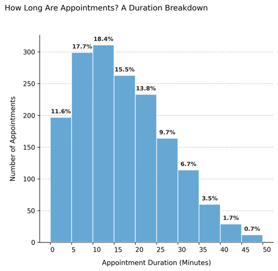
Explanation:

• Durations follow a Beta(1.48, 3.6) distribution scaled to 0–60 min.

• This yields short right-skewed sessions with typical times between 10 – 25 min.

• Derived from Tai-Seale et al. (2007), these values approximate observed patterns in primary care.

This distribution interacts with arrival times to shape overall waiting patterns — even when punctuality is ideal, short or long sessions can affect subsequent delays.

---

Example 2 – Frequent late arrivals

A clinic where patients often arrive after their scheduled time, causing downstream delays.

sched_late = AppointmentScheduler(
    date_ranges=[("2024-01-01", "2024-03-31")],
    ref_date="2024-03-15",
    check_in_time_mean=5,   # average 5 min late
    fill_rate=0.85
)

slots_df, appts_df, patients_df = sched_late.generate()

plot_arrival_time_distribution(appts_df)
plot_waiting_time_distribution(appts_df)

Output preview:

1. Arrival time distribution – Skewed toward later arrivals, showing frequent tardiness.
   

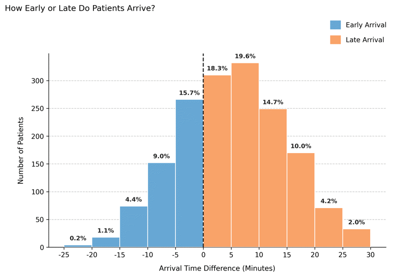
2. Waiting time distribution – Broader and asymmetric, as delays accumulate downstream.
   

Interpretation:
When patients arrive late on average, waiting times become irregular and less predictable.
This scenario represents real clinics struggling with punctuality compliance, where even minor delays propagate through the day.

---

Example 3 – High-efficiency morning clinic

A tightly managed setting where patients arrive well in advance, minimizing idle time between consultations.

sched_fast = AppointmentScheduler(
    date_ranges=[("2024-01-01", "2024-03-31")],
    ref_date="2024-03-15",
    check_in_time_mean=-15,  # very early arrivals
    fill_rate=0.9
)

slots_df, appts_df, patients_df = sched_fast.generate()

plot_arrival_time_distribution(appts_df)
plot_waiting_time_distribution(appts_df)

Output preview:

1. Arrival time distribution – Concentrated around −15 minutes, most patients early.
   

2. Waiting time distribution – Lower median wait (< 3 min) due to synchronized readiness.
   

Interpretation:
Early arrivals and steady throughput yield minimal idle time and consistent session flow.
This configuration suits high-volume diagnostics or vaccination sessions where speed and regularity are prioritized.

---

Summary

Scenario	check_in_time_mean	Behavior	Typical waiting time	Operational impact
Standard	−10 min	Early punctuality	~5 min	Balanced and efficient
Late arrivals	+5 min	Patients often delayed	>10 min	Variable and delayed
Fast clinic	−15 min	Very early arrivals	<3 min	Smooth and consistent

---

Notes

• Arrival-time patterns directly control waiting-time distributions.

• Appointment durations are fixed by the internal Beta(1.48, 3.6) model, independent of punctuality.

• Flow stability depends on the interaction between punctuality, duration variability, and fill rate.

---

Next Steps

• Examine Appointments table for time variables.

• Review Randomness and variability to understand stochastic components.

• Explore Attendance behavior to connect punctuality with attendance outcomes.

• Revisit Patient Flow and Demographic Structure to analyze how demographic traits affect punctuality trends.